Critical Points and the Hessian

Critical points from the gradient

A critical point of a differentiable function $f(x,y)$ is a point $(x_0,y_0)$ where the gradient vanishes:

$$\nabla f(x_0,y_0)=\left(\frac{\partial f}{\partial x},\frac{\partial f}{\partial y}\right)=(0,0).$$

See Directional Derivatives and the Gradient for the full derivation of $\nabla f$ and the formula $D_{\mathbf{u}}f=\nabla f\cdot \mathbf{u}$. That formula has an immediate consequence here: if $\nabla f=0$, then $D_{\mathbf{u}}f=0\cdot \mathbf{u}=0$ for every unit vector $\mathbf{u}$. The directional derivative is zero in every direction. Geometrically, the surface $z=f(x,y)$ is momentarily flat at $(x_0,y_0)$ --- it has a horizontal tangent plane.

But “flat” is ambiguous. A hilltop is flat at the summit (local maximum). A valley floor is flat at the bottom (local minimum). A mountain pass is flat at the saddle --- it curves up in one direction and down in another (saddle point). The gradient alone cannot distinguish these cases because it only captures first-order behaviour. To classify a critical point, we need second-order information: the second partial derivatives of $f$.

Second-order Taylor expansion at a critical point

The tool for extracting second-order behaviour is the Taylor expansion --- the approximation of a function by a polynomial that matches the function’s value and derivatives at a point. For a function of two variables, the second-order Taylor expansion of $f$ around the point $(x_0,y_0)$ is

$$f(x_0+h,y_0+k)\approx f(x_0,y_0)+f_{x}h+f_{y}k+\frac{1}{2}\left(f_{xx}{h}^2+2f_{xy}hk+f_{yy}{k}^2\right),$$

where all partial derivatives are evaluated at $(x_0,y_0)$, $h=x-x_0$ is the displacement in $x$, and $k=y-y_0$ is the displacement in $y$. The notation $f_{xx}=\frac{{\partial }^{2}f}{\partial x^2}$, $f_{xy}=\frac{{\partial }^{2}f}{\partial x\partial y}$, and $f_{yy}=\frac{{\partial }^{2}f}{\partial y^2}$ denotes the second partial derivatives --- derivatives of derivatives.

At a critical point, $f_x=0$ and $f_y=0$, so the linear terms vanish. Subtracting the constant $f(x_0,y_0)$, the change in function value is controlled entirely by the quadratic form --- a homogeneous polynomial of degree 2 in $h$ and $k$:

$$\Delta f\approx \frac{1}{2}\left(A{h}^2+2Bhk+C{k}^2\right),$$

where we introduce the shorthand

$$A=f_{xx}(x_0,y_0),B=f_{xy}(x_0,y_0),C=f_{yy}(x_0,y_0).$$

A quadratic form is an expression of the type $\alpha h^2+\beta hk+\gamma k^2$ --- a polynomial where every term has total degree exactly 2. Quadratic forms are the two-variable analogue of $a{x}^2$ in single-variable calculus: they capture the curvature of the function.

The key insight

Near a critical point, the function’s behaviour is determined by the sign of the quadratic form $A{h}^2+2Bhk+C{k}^2$. If this form is always positive (for every displacement $(h,k)\ne (0,0)$), the critical point is a local minimum. If always negative, a local maximum. If it changes sign depending on direction, a saddle point.

Quadratic form as matrix product: the Hessian

The quadratic form $A{h}^2+2Bhk+C{k}^2$ can be written as a matrix product. Define the column vector $\mathbf{v}=\left(\begin{array}{c}h\\ k\end{array}\right)$ and the $2\times 2$ matrix

$$H=\left(\begin{array}{cc}A& B\\ B& C\end{array}\right)=\left(\begin{array}{cc}{f}_{xx}& f_{xy}\\ f_{xy}& f_{yy}\end{array}\right).$$

Then

$${\mathbf{v}}^{T}H\mathbf{v}=\left(\begin{array}{cc}h& k\end{array}\right)\left(\begin{array}{cc}A& B\\ B& C\end{array}\right)\left(\begin{array}{c}h\\ k\end{array}\right)=A{h}^2+2Bhk+C{k}^2,$$

and so $\Delta f\approx \frac{1}{2}{\mathbf{v}}^{T}H\mathbf{v}$.

The matrix $H$ is the Hessian matrix of $f$ at the critical point --- the matrix of all second partial derivatives. It is named after the German mathematician Ludwig Otto Hesse (1811—1874), who introduced it in the context of algebraic geometry.

Notice that $B=f_{xy}$ appears in both off-diagonal positions. This is because of Clairaut’s theorem (also called Schwarz’s theorem): if the second partial derivatives $f_{xy}$ and $f_{yx}$ are both continuous, then $f_{xy}=f_{yx}$ --- the order of differentiation does not matter. This symmetry $f_{xy}=f_{yx}$ is what makes $H$ a symmetric matrix (a matrix equal to its own transpose: $H=H^T$).

Notation bridge

MIT 18.02 uses $A=f_{xx}$, $B=f_{xy}$, $C=f_{yy}$ and checks $AC-B^2$. Politecnico di Torino teaches this as the Hessian matrix $H$, checking $\det (H)$ and eigenvalues. Same object, same test, different packaging.

The second-derivative test: classification table

The sign behaviour of the quadratic form ${\mathbf{v}}^{T}H\mathbf{v}$ determines the nature of the critical point. The classification depends on the determinant of the Hessian, $\det (H)=AC-B^2$, and the sign of $A=f_{xx}$:

$\det (H)=AC-B^2$	$A$	Classification
$>0$	$>0$	Local minimum
$>0$	$<0$	Local maximum
$<0$	any	Saddle point
$=0$	any	Degenerate (test inconclusive)

Why these conditions work

• When $\det (H)>0$ and $A>0$: both eigenvalues are positive (see next section), so the quadratic form is always positive --- the surface curves upward in every direction. Local minimum.
• When $\det (H)>0$ and $A<0$: both eigenvalues are negative, so the quadratic form is always negative --- the surface curves downward in every direction. Local maximum.
• When $\det (H)<0$: the eigenvalues have opposite signs, so the quadratic form is positive in some directions and negative in others --- the surface curves up one way and down another. Saddle point.
• When $\det (H)=0$: at least one eigenvalue is zero, and the second-order information is insufficient. The point could be a minimum, maximum, saddle, or something more exotic. Higher-order derivatives are needed. This case is called degenerate.

A quadratic form that is always positive (for all non-zero $\mathbf{v}$) is called positive definite. Always negative: negative definite. Takes both signs: indefinite. Has a zero but is otherwise non-negative (or non-positive): semi-definite.

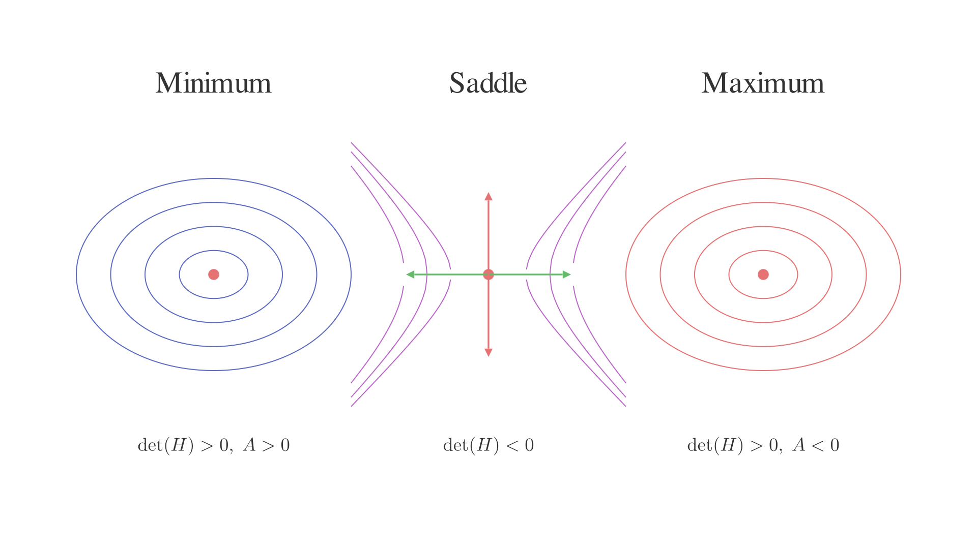
The diagram below shows the contour patterns for each case: elliptical contours closing around a minimum (left), hyperbolic contours at a saddle with eigenvector arrows showing the up/down directions (center), and elliptical contours around a maximum (right).

Eigenvalue connection

The classification table above is really a statement about the eigenvalues of $H$. An eigenvalue $\lambda$ of a matrix $M$ is a scalar such that $M\mathbf{w}=\lambda \mathbf{w}$ for some non-zero vector $\mathbf{w}$ (called an eigenvector) --- the matrix acts on $\mathbf{w}$ by simply scaling it. The eigenvalues of a $2\times 2$ matrix are the roots of its characteristic polynomial $\det (M-\lambda I)=0$.

Because $H$ is symmetric, a powerful result from linear algebra guarantees that its eigenvalues are well-behaved:

Spectral Theorem (for real symmetric matrices). Every real symmetric matrix has all real eigenvalues and can be diagonalized by an orthogonal matrix (a matrix whose columns are mutually perpendicular unit vectors). In other words, symmetric matrices have no complex eigenvalues, and their eigenvectors can be chosen to be orthogonal.

For our $2\times 2$ Hessian with eigenvalues ${\lambda }_1$ and ${\lambda }_2$, two standard facts from linear algebra connect eigenvalues to the determinant and trace:

$$\det (H)={\lambda }_1{\lambda }_2,\text{tr}(H)={\lambda }_1+{\lambda }_2=A+C.$$

The trace $\text{tr}(H)$ is the sum of the diagonal entries. Now the classification table translates directly into eigenvalue language:

Eigenvalue condition	Quadratic form	Critical point
${\lambda }_1>0,{\lambda }_2>0$	Positive definite	Local minimum
${\lambda }_1<0,{\lambda }_2<0$	Negative definite	Local maximum
${\lambda }_1$ and ${\lambda }_2$ have opposite signs	Indefinite	Saddle point
${\lambda }_1=0$ or ${\lambda }_2=0$	Semi-definite	Degenerate

When both eigenvalues are positive, their product $\det (H)={\lambda }_1{\lambda }_2>0$ and $A=f_{xx}>0$ (because $A$ is the $(1,1)$ entry of a positive-definite matrix). When both are negative, the product is still positive but $A<0$. When they have opposite signs, the product is negative. This is exactly the $AC-B^2$ test in the previous section.

The eigenvalue perspective also reveals the principal directions of curvature: the eigenvectors of $H$ point in the directions along which the surface curves the most and the least. The corresponding eigenvalues are the curvatures in those directions.

Worked examples

Example 1: $f(x,y)=x^2+y^2$ (local minimum)

Gradient.

$$\nabla f=(2x,2y).$$

Setting $\nabla f=(0,0)$ gives the critical point $(0,0)$.

Hessian.

$$f_{xx}=2,f_{xy}=0,f_{yy}=2,H=\left(\begin{array}{cc}2& 0\\ 0& 2\end{array}\right).$$

Determinant and classification.

$$\det (H)=2\cdot 2-0^2=4>0,A=2>0.$$

$\det (H)>0$ and $A>0$: local minimum.

Eigenvalues. ${\lambda }_1=2$, ${\lambda }_2=2$. Both positive, confirming positive definiteness. The surface is a paraboloid opening upward.

---

Example 2: $f(x,y)=-x^2-y^2$ (local maximum)

Gradient.

$$\nabla f=(-2x,-2y).$$

Critical point: $(0,0)$.

Hessian.

$$f_{xx}=-2,f_{xy}=0,f_{yy}=-2,H=\left(\begin{array}{cc}-2& 0\\ 0& -2\end{array}\right).$$

Determinant and classification.

$$\det (H)=(-2)(-2)-0^2=4>0,A=-2<0.$$

$\det (H)>0$ and $A<0$: local maximum.

Eigenvalues. ${\lambda }_1=-2$, ${\lambda }_2=-2$. Both negative, confirming negative definiteness. The surface is an inverted paraboloid.

---

Example 3: $f(x,y)=x^2-y^2$ (saddle point)

Gradient.

$$\nabla f=(2x,-2y).$$

Critical point: $(0,0)$.

Hessian.

$$f_{xx}=2,f_{xy}=0,f_{yy}=-2,H=\left(\begin{array}{cc}2& 0\\ 0& -2\end{array}\right).$$

Determinant and classification.

$$\det (H)=2\cdot (-2)-0^2=-4<0.$$

$\det (H)<0$: saddle point, regardless of $A$.

Eigenvalues. ${\lambda }_1=2$, ${\lambda }_2=-2$. Opposite signs confirm indefiniteness. Along the $x$-axis the surface curves up ($+2x^2$); along the $y$-axis it curves down ($-2y^2$). The surface is a hyperbolic paraboloid --- the classic saddle shape.

---

Example 4: $f(x,y)=x^3$ (degenerate)

Gradient.

$$\nabla f=(3x^2,0).$$

Setting $\nabla f=(0,0)$: $3x^2=0$ gives $x=0$, and $y$ is free --- but $f_y=0$ everywhere, so the entire $y$-axis consists of critical points. Take $(0,0)$.

Hessian.

$$f_{xx}=6x,f_{xy}=0,f_{yy}=0,H{|}_{(0,0)}=\left(\begin{array}{cc}0& 0\\ 0& 0\end{array}\right).$$

Determinant and classification.

$$\det (H)=0\cdot 0-0^2=0.$$

$\det (H)=0$: degenerate --- the second-derivative test is inconclusive.

Eigenvalues. ${\lambda }_1=0$, ${\lambda }_2=0$. Both zero: the Hessian carries no curvature information at all.

What actually happens. Along the $x$-axis, $f(x,0)=x^3$, which is increasing (not a minimum or maximum). The origin is an inflection point of the single-variable slice $x\mapsto x^3$. To resolve degenerate cases, one must examine third- or higher-order derivatives, or analyse the function directly. The second-derivative test simply cannot help here.

See also

• Directional Derivatives and the Gradient --- the gradient whose vanishing defines critical points
• Lagrange Multipliers --- constrained optimization, which finds critical points of $f$ subject to a constraint $g=k$
• Tangent Vectors and the Unit Normal on Graph Surfaces --- tangent planes and the normal vector for surfaces $z=f(x,y)$; the tangent plane is horizontal at critical points