Directional Derivatives and the Gradient

The question

Partial derivatives measure how a function $f(x,y)$ changes when you move along the coordinate axes --- $\frac{\partial f}{\partial x}$ holds $y$ fixed and varies $x$, while $\frac{\partial f}{\partial y}$ holds $x$ fixed and varies $y$. But the coordinate axes are arbitrary. There is nothing physically special about the $x$- or $y$-direction; they are an artifact of the coordinate system we happened to choose.

The natural question: what is the rate of change of $f$ in an arbitrary direction? If you stand at a point $(x_0,y_0)$ and walk in a direction that is neither pure $x$ nor pure $y$, how fast does $f$ change per unit distance traveled?

The answer is the directional derivative, and the tool that makes it computable is the gradient vector $\nabla f$. Both emerge from a single application of the chain rule.

Setup: walking in direction $\mathbf{u}$

Choose a unit vector $\mathbf{u}=(a,b)$ with $\Vert \mathbf{u}\Vert =\sqrt{a^2+b^2}=1$. A unit vector is a vector of length 1 --- it specifies a direction without any scale ambiguity.

Starting at the point $P=(x_0,y_0)$, walk in the direction $\mathbf{u}$. Your position after traveling a distance $s$ along this direction is

$$\mathbf{r}(s)=(x_0+as,y_0+bs).$$

This is a straight line through $P$ in the direction $\mathbf{u}$, parametrized by arc length --- the parameter $s$ measures actual distance traveled, not some arbitrary quantity. See Arc-Length Parametrization for why this matters: because $\mathbf{u}$ is a unit vector, $\Vert \frac{d\mathbf{r}}{ds}\Vert =\Vert \mathbf{u}\Vert =1$, so the parametrization has unit speed and $s$ is genuinely distance.

From this parametrization, the components of position are functions of $s$:

$$x(s)=x_0+as,y(s)=y_0+bs.$$

Their derivatives with respect to $s$ are simply the components of $\mathbf{u}$:

$$\frac{dx}{ds}=a,\frac{dy}{ds}=b.$$

The chain rule derivation

Now consider the scalar function $w=f(x,y)$ evaluated along this line. As $s$ varies, both $x$ and $y$ change, so $w$ is a composite function: $w(s)=f(x(s),y(s))$.

The multivariable chain rule tells us how to differentiate a composite function. If $w=f(x,y)$ where $x$ and $y$ are both differentiable functions of a single parameter $s$, then

$$\frac{dw}{ds}=\frac{\partial f}{\partial x}\frac{dx}{ds}+\frac{\partial f}{\partial y}\frac{dy}{ds}.$$

This is the sum of two contributions: the rate of change of $f$ due to $x$ changing (weighted by how fast $x$ changes with $s$) plus the rate of change of $f$ due to $y$ changing (weighted by how fast $y$ changes with $s$). It generalizes the single-variable chain rule $\frac{dw}{ds}=\frac{dw}{dx}\frac{dx}{ds}$ to the case where $w$ depends on multiple intermediate variables.

Substituting $\frac{dx}{ds}=a$ and $\frac{dy}{ds}=b$:

$$\frac{dw}{ds}=f_x\cdot a+f_y\cdot b,$$

where $f_x=\frac{\partial f}{\partial x}$ and $f_y=\frac{\partial f}{\partial y}$ are the partial derivatives of $f$, evaluated at $(x_0,y_0)$.

This quantity $\frac{dw}{ds}{|}_{s=0}$ is the directional derivative of $f$ at $P$ in the direction $\mathbf{u}$, written $D_{\mathbf{u}}f(P)$.

Concrete example

Take $f(x,y)=x^{2}y+y^3$. Compute the directional derivative at the point $(1,2)$ in the direction $\mathbf{u}=\left(\frac{3}{5},\frac{4}{5}\right)$ (which is a unit vector since $\sqrt{9/25+16/25}=1$).

Step 1: Compute the partial derivatives.

$$f_x=\frac{\partial }{\partial x}(x^{2}y+y^3)=2xy,f_y=\frac{\partial }{\partial y}(x^{2}y+y^3)=x^2+3y^2.$$

Step 2: Evaluate at $(1,2)$.

$$f_x(1,2)=2\cdot 1\cdot 2=4,f_y(1,2)=1^2+3\cdot 2^2=1+12=13.$$

Step 3: Apply the formula.

$$D_{\mathbf{u}}f(1,2)=f_x\cdot a+f_y\cdot b=4\cdot \frac{3}{5}+13\cdot \frac{4}{5}=\frac{12}{5}+\frac{52}{5}=\frac{64}{5}=\mathrm{12.8.}$$

The function $f$ increases at a rate of 12.8 units per unit distance when you walk from $(1,2)$ in the direction $\left(\frac{3}{5},\frac{4}{5}\right)$.

Repackaging as a dot product: the gradient

Look at the formula again:

$$D_{\mathbf{u}}f=f_x\cdot a+f_y\cdot b.$$

The right side is a dot product --- the sum of component-wise products of two vectors. The dot product of vectors $\mathbf{v}=(v_1,v_2)$ and $\mathbf{w}=(w_1,w_2)$ is $\mathbf{v}\cdot \mathbf{w}=v_1{w}_1+v_2{w}_2$. Recognizing this pattern, define the gradient of $f$:

$$\nabla f=\left(\frac{\partial f}{\partial x},\frac{\partial f}{\partial y}\right)=(f_x,f_y).$$

The symbol $\nabla$ is called “nabla” or “del.” The gradient $\nabla f$ is a vector whose components are the partial derivatives of $f$. It is not new mathematics --- it is a repackaging of information we already had (the partial derivatives) into a single vector object that makes the directional derivative formula clean:

$$\boxed{D_{\mathbf{u}}f=\nabla f\cdot \mathbf{u}.}$$

The directional derivative in any direction $\mathbf{u}$ is the dot product of the gradient with $\mathbf{u}$.

The gradient in higher dimensions

Everything generalizes immediately. For $f(x_1,x_2,\dots ,x_n)$, the gradient is $\nabla f=\left(\frac{\partial f}{\partial x_1},\frac{\partial f}{\partial x_2},\dots ,\frac{\partial f}{\partial x_n}\right)$, and $D_{\mathbf{u}}f=\nabla f\cdot \mathbf{u}$ for any unit vector $\mathbf{u}\in {\mathbb{R}}^n$.

For the example above: $\nabla f(1,2)=(4,13)$, and $D_{\mathbf{u}}f=(4,13)\cdot \left(\frac{3}{5},\frac{4}{5}\right)=\frac{64}{5}$. Same answer, but now the computation has a geometric shape.

Three geometric consequences

The power of the dot product formula comes from a fundamental identity. For any two vectors $\mathbf{a}$ and $\mathbf{b}$, the dot product satisfies

$$\mathbf{a}\cdot \mathbf{b}=\Vert \mathbf{a}\Vert \Vert \mathbf{b}\Vert \cos \theta ,$$

where $\theta$ is the angle between the two vectors. Since $\mathbf{u}$ is a unit vector ($\Vert \mathbf{u}\Vert =1$), this simplifies to

$$D_{\mathbf{u}}f=\nabla f\cdot \mathbf{u}=\Vert \nabla f\Vert \cos \theta ,$$

where $\theta$ is the angle between $\nabla f$ and $\mathbf{u}$. The directional derivative depends only on the magnitude of the gradient and the angle $\theta$. This gives three immediate results:

Maximum rate of increase

When $\theta =0$ (you walk in the same direction as $\nabla f$), $\cos 0=1$ and

$$D_{\mathbf{u}}f=\Vert \nabla f\Vert .$$

This is the largest possible directional derivative. The gradient points in the direction of steepest ascent, and its magnitude $\Vert \nabla f\Vert$ is the rate of that steepest ascent.

Maximum rate of decrease

When $\theta =\pi$ (you walk directly opposite to $\nabla f$), $\cos \pi =-1$ and

$$D_{\mathbf{u}}f=-\Vert \nabla f\Vert .$$

This is the most negative directional derivative. Walking opposite the gradient gives the steepest descent.

Zero change

When $\theta =\frac{\pi }{2}$ (you walk perpendicular to $\nabla f$), $\cos \frac{\pi }{2}=0$ and

$$D_{\mathbf{u}}f=0.$$

Walking perpendicular to the gradient, $f$ does not change at all (to first order). This is not a coincidence --- it is the key to the next section.

The punchline: the gradient is normal to level curves

A level curve (also called a contour) of $f(x,y)$ is a curve in the $xy$-plane along which $f$ takes a constant value: $\{(x,y):f(x,y)=k\}$ for some constant $k$. For example, the level curves of $f(x,y)=x^2+y^2$ are circles centered at the origin.

The gradient is perpendicular to level curves

At any point on a level curve $f(x,y)=k$, the gradient $\nabla f$ is perpendicular (normal) to the level curve.

Proof. Let $\mathbf{u}$ be a unit tangent vector to the level curve at some point $P$. “Tangent to the level curve” means $\mathbf{u}$ points along the curve --- in a direction where $f$ stays constant. Since $f$ does not change along the level curve, the rate of change of $f$ in the direction $\mathbf{u}$ is zero:

$D_{\mathbf{u}}f=0.$

But $D_{\mathbf{u}}f=\nabla f\cdot \mathbf{u}$. So

$\nabla f\cdot \mathbf{u}=0.$

A dot product of zero means the two vectors are orthogonal (perpendicular), provided neither is the zero vector. Therefore $\nabla f\perp \mathbf{u}$. Since this holds for every tangent direction $\mathbf{u}$ to the level curve, $\nabla f$ is normal to the level curve at $P$. $■$

This is one of the most important results in multivariable calculus. It connects two seemingly different ideas --- the algebraic object $\nabla f$ (a vector of partial derivatives) and the geometric object “level curve” (a contour of constant $f$) --- through the directional derivative.

The gradient does double duty: it tells you the direction of steepest increase and it tells you which way is “outward” from a level curve. These are the same thing --- the steepest way to increase $f$ is to walk directly away from the current contour toward higher-valued contours.

Worked example: gradient perpendicular to a circle

Take $f(x,y)=x^2+y^2$.

Step 1: Compute the gradient.

$$\nabla f=(2x,2y).$$

Step 2: Evaluate at the point $(1,1)$.

$$\nabla f(1,1)=(2,2).$$

Step 3: Identify the level curve through $(1,1)$.

$$f(1,1)=1^2+1^2=2,$$

so the level curve is $x^2+y^2=2$, a circle of radius $\sqrt{2}$ centered at the origin.

Step 4: Find a tangent vector to the circle at $(1,1)$.

The circle $x^2+y^2=2$ can be parametrized as $\mathbf{r}(t)=(\sqrt{2}\cos t,\sqrt{2}\sin t)$. The point $(1,1)=(\sqrt{2}\cos \frac{\pi }{4},\sqrt{2}\sin \frac{\pi }{4})$ corresponds to $t=\frac{\pi }{4}$. The tangent vector is

$${\mathbf{r}}^{\prime }(t)=(-\sqrt{2}\sin t,\sqrt{2}\cos t).$$

At $t=\frac{\pi }{4}$:

$${\mathbf{r}}^{\prime }\left(\frac{\pi }{4}\right)=(-\sqrt{2}\cdot \frac{\sqrt{2}}{2},\sqrt{2}\cdot \frac{\sqrt{2}}{2})=(-1,1).$$

Step 5: Verify perpendicularity.

$$\nabla f(1,1)\cdot {\mathbf{r}}^{\prime }\left(\frac{\pi }{4}\right)=(2,2)\cdot (-1,1)=2\cdot (-1)+2\cdot 1=-2+2=0.$$

The dot product is zero, confirming that the gradient $(2,2)$ is perpendicular to the tangent direction $(-1,1)$ at the point $(1,1)$.

Geometric picture

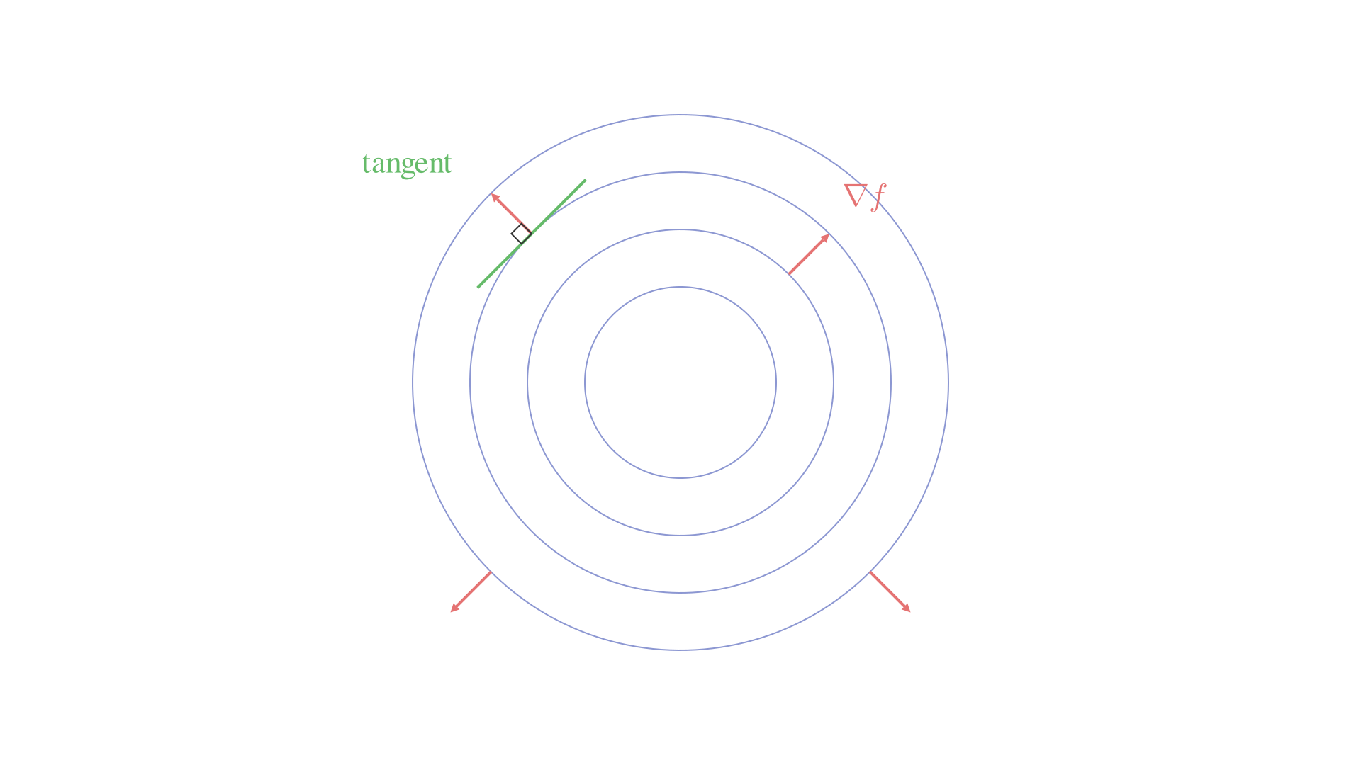
At every point on the circle $x^2+y^2=2$, the gradient $\nabla f=(2x,2y)$ points radially outward from the origin, while the tangent to the circle points along the circumference. Radii and tangent lines of a circle are always perpendicular --- the gradient-level-curve relationship is the general version of this familiar geometric fact.

The diagram below shows concentric level curves of $f(x,y)=x^2+y^2$ with gradient arrows (red) pointing radially outward. At the upper-left point, a green tangent segment and a right-angle marker confirm the perpendicularity.

See also

• Arc-Length Parametrization --- the arc-length parametrization of straight lines is the foundation of the directional derivative definition
• Tangent Vectors and the Unit Normal on Graph Surfaces --- tangent planes and normals for surfaces $z=f(x,y)$, where the gradient appears in the normal vector formula
• Critical Points and the Hessian --- what happens when $\nabla f=0$ (the gradient vanishes): critical points, and the second-derivative test for classifying them
• Lagrange Multipliers --- uses the gradient-perpendicular-to-level-curves result to optimize $f$ subject to constraints