IEJoin Algorithm

IEJoin (Inequality Join) is an algorithm for efficiently joining two relations on inequality conditions — predicates like l.a > r.b AND l.c < r.d that standard hash joins and sort-merge joins cannot handle. It was introduced in:

Khayyat, Z., Lucia, W., Singh, M., Ouzzani, M., Papotti, P., Quiane-Ruiz, J., Tang, N., Kalnis, P. “Lightning Fast and Space Efficient Inequality Joins.” Proceedings of the VLDB Endowment, Vol. 8, No. 13, 2015.

Prerequisites

11 - Join algorithms — equi-join algorithms and their I/O cost models

ASOF Join — the specialized join that IEJoin generalizes

The Problem

Inequality joins appear in temporal databases (find overlapping events), data cleaning (find tuples violating constraints), and spatial queries (find nearby points). Standard database engines handle them poorly:

Nested loop join: $O (m \times n)$ — checks every pair. Works, but quadratic.
Cartesian product + filter: What most optimizers actually do. Same quadratic cost, often worse due to materialization overhead.
Index-based (B+-tree, R-tree, GiST): Requires building indices on each attribute. Index construction itself can exceed the join cost for large relations. R-trees (spatial index structures) suffer random I/O on unclustered data.

The paper’s motivating story: “Bob” tried running a two-condition inequality self-join ( $Q_{t}$ : find West-Coast transactions that last longer and cost less than East-Coast transactions) on five different database systems. None could finish efficiently — they all fell back to Cartesian product followed by selection.

Core Insight

IEJoin avoids materializing the Cartesian product by exploiting the sortedness of the join attributes:

# The three data structures that make IEJoin work:
 
# 1. Sort all tuples by each join attribute independently
sorted_by_time = sort(tuples, key=lambda t: t.time)    # e.g. [s3, s4, s1, s2]
sorted_by_cost = sort(tuples, key=lambda t: t.cost)    # e.g. [s4, s1, s3, s2]
 
# 2. Build a permutation array: for each tuple in cost-sorted order,
#    record its position in time-sorted order. This bridges the two
#    sort orders without materializing pairs.
permutation = [position_in_sorted_by_time(t) for t in sorted_by_cost]
 
# 3. A visited bit-array tracks which time-sorted positions have been
#    "activated" so far, enabling efficient result enumeration.
visited = [False] * len(tuples)

The key property: sorting encodes one condition into the iteration order, and the permutation array encodes the other condition into position lookups. This avoids comparing both attributes for every pair — but it doesn’t eliminate the inner loop entirely (see “What about the inner loop?” below).

Worked Example: Self-Join (IESelfJoin)

Consider a self-join on a west transactions table with two inequality conditions:

SELECT a.id, b.id
FROM west a, west b
WHERE a.time > b.time AND a.cost < b.cost;

“Find pairs where one transaction happened later but cost less.”

Input Data

id	time	cost
s1	100	6
s2	140	11
s3	80	10
s4	90	5

Step 1 — Sort and Build Data Structures

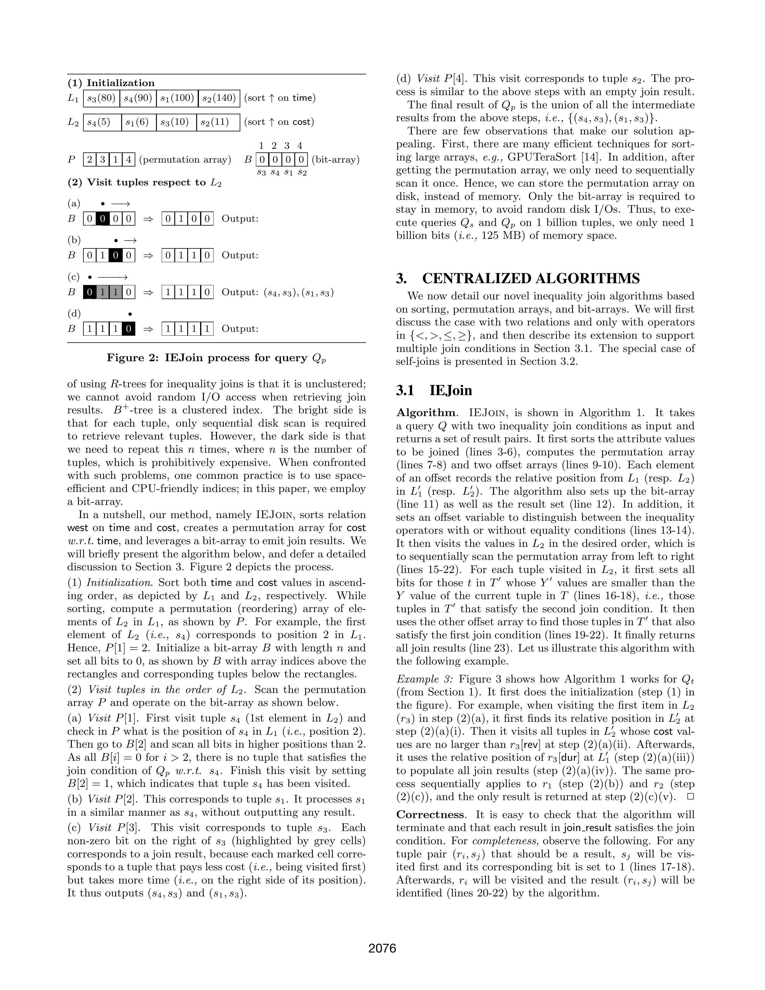
Figure 2 from Khayyat et al. (VLDB 2015): The IEJoin initialization and result enumeration for a self-join. Left (1): the sorted arrays, permutation array, and bit-array after initialization. Right (2): the main loop iterating in cost order.

The following is runnable Python — paste it into a REPL to see every intermediate step:

from dataclasses import dataclass
 
@dataclass
class Txn:
    id: str
    time: int
    cost: int
 
tuples = [Txn("s1", 100, 6), Txn("s2", 140, 11), Txn("s3", 80, 10), Txn("s4", 90, 5)]
 
# Sort by time (ascending). The INDEX in this list encodes the time
# ranking: index 0 = earliest, index 3 = latest.
sorted_by_time = sorted(tuples, key=lambda t: t.time)
print("sorted_by_time:")
for i, t in enumerate(sorted_by_time):
    print(f"  index {i}: {t.id} (time={t.time})")
# index 0: s3 (time=80)
# index 1: s4 (time=90)
# index 2: s1 (time=100)
# index 3: s2 (time=140)
 
# Build a lookup: given a tuple, what is its index in sorted_by_time?
time_rank = {t.id: i for i, t in enumerate(sorted_by_time)}
print(f"\ntime_rank: {time_rank}")
# {'s3': 0, 's4': 1, 's1': 2, 's2': 3}
 
# Sort by cost (ascending). This determines the ORDER in which the
# main loop processes tuples — lowest cost first.
sorted_by_cost = sorted(tuples, key=lambda t: t.cost)
print("\nsorted_by_cost (= processing order for main loop):")
for i, t in enumerate(sorted_by_cost):
    print(f"  process {i}: {t.id} (cost={t.cost})")
# process 0: s4 (cost=5)   ← processed first (lowest cost)
# process 1: s1 (cost=6)
# process 2: s3 (cost=10)
# process 3: s2 (cost=11)  ← processed last (highest cost)

Now the permutation array. Why is it in cost order? Because the main loop iterates through tuples from lowest cost to highest. For each tuple it processes, it needs to know where that tuple sits in the time ranking. The permutation array answers exactly that question: permutation[i] = “the tuple I’m processing in iteration i has this time-rank.”

# The permutation array: read sorted_by_cost in order, look up each
# tuple's position in sorted_by_time.
permutation = [time_rank[t.id] for t in sorted_by_cost]
print(f"\npermutation: {permutation}")
# [1, 2, 0, 3]
# Meaning:
#   iteration 0 processes s4 → s4's time-rank is 1
#   iteration 1 processes s1 → s1's time-rank is 2
#   iteration 2 processes s3 → s3's time-rank is 0
#   iteration 3 processes s2 → s2's time-rank is 3

Step 2 — The Main Loop

The loop iterates over permutation (i.e., over tuples in cost order, lowest cost first). It maintains a marked boolean array indexed by time-rank. On each iteration:

Check for matches: look at marked for any True at positions above the current tuple’s time-rank. Each True represents a tuple that was processed in an earlier iteration (= has a lower cost value) and has a higher time-rank (= happened later). That’s both join conditions satisfied.
Mark: set marked[time_rank] = True so future iterations can find this tuple.

The marked array only accumulates — bits are set to True and never cleared. It’s not a stack, nothing gets popped.

n = len(sorted_by_time)
marked = [False] * n
results = []
 
for i, time_pos in enumerate(permutation):
    current = sorted_by_cost[i]
    print(f"\n--- Iteration {i}: processing {current.id} "
          f"(cost={current.cost}, time={current.time}, time_rank={time_pos}) ---")
    print(f"  marked before: {marked}")
 
    # Check: are there any True entries at positions ABOVE time_pos?
    # Each one is a match — a tuple with lower cost AND later time.
    for j in range(time_pos + 1, n):
        if marked[j]:
            match = sorted_by_time[j]
            print(f"  MATCH: marked[{j}] is True → {match.id} "
                  f"(time={match.time}, cost={match.cost})")
            print(f"    {match.id}.time={match.time} > {current.id}.time={current.time}  ✓")
            print(f"    {match.id}.cost={match.cost} < {current.id}.cost={current.cost}  ✓")
            results.append((match.id, current.id))
 
    if not any(marked[j] for j in range(time_pos + 1, n)):
        print(f"  No True in marked[{time_pos+1}:] → no matches")
 
    # Mark this tuple's time-rank so future iterations can find it
    marked[time_pos] = True
    print(f"  marked after:  {marked}")
 
print(f"\nFinal results: {results}")

Running this prints:

--- Iteration 0: processing s4 (cost=5, time=90, time_rank=1) ---
  marked before: [False, False, False, False]
  No True in marked[2:] → no matches
  marked after:  [False, True, False, False]

--- Iteration 1: processing s1 (cost=6, time=100, time_rank=2) ---
  marked before: [False, True, False, False]
  No True in marked[3:] → no matches
  marked after:  [False, True, True, False]

--- Iteration 2: processing s3 (cost=10, time=80, time_rank=0) ---
  marked before: [False, True, True, False]
  MATCH: marked[1] is True → s4 (time=90, cost=5)
    s4.time=90 > s3.time=80  ✓
    s4.cost=5 < s3.cost=10  ✓
  MATCH: marked[2] is True → s1 (time=100, cost=6)
    s1.time=100 > s3.time=80  ✓
    s1.cost=6 < s3.cost=10  ✓
  marked after:  [True, True, True, False]

--- Iteration 3: processing s2 (cost=11, time=140, time_rank=3) ---
  marked before: [True, True, True, False]
  No True in marked[4:] → no matches
  marked after:  [True, True, True, True]

Final results: [('s4', 's3'), ('s1', 's3')]

Why This Works

The loop gets both join conditions for free from the data structure design:

Cost condition (a.cost < b.cost): the loop processes tuples from lowest cost to highest. Any tuple already marked was processed in an earlier iteration, so it has a lower cost value than the current tuple.
Time condition (a.time > b.time): the marked array is indexed by time-rank. A True at a position above the current position means that tuple has a higher time-rank — i.e., it happened later. Checking marked[time_pos+1:] finds exactly those tuples.

The permutation array is the bridge: it lets the loop iterate in cost order while checking time-rank positions. Without it, you’d need to compare both attributes for every pair.

What About the Inner Loop?

Look at the main loop again — there’s a nested for j in range(time_pos + 1, n) inside the outer for i in range(n). That’s still an inner loop. In the worst case (every tuple matches every other tuple), the inner loop scans the entire marked array on each outer iteration — $O (n)$ inner work × $n$ outer iterations = $O (n^{2})$ total. So IEJoin is not subquadratic in the worst case.

What it does avoid is the Cartesian product materialization. The naive approach (FROM T a, T b WHERE a.time > b.time AND a.cost < b.cost) first materializes all $n^{2}$ pairs as intermediate rows, then filters. IEJoin never materializes non-matching pairs — the inner loop scans a compact bit-array (one bit per tuple, not one full row per tuple), and the Bloom filter optimization (see below) lets it skip large empty chunks entirely.

The real complexity is output-sensitive: $O (n lo g n + n + ∣ output ∣)$ , where $∣ output ∣$ is the number of matching pairs. When selectivity is low (few matches), most inner loop iterations scan empty bits and the Bloom filter skips them in bulk. When selectivity is high (many matches), the $O (n^{2})$ is unavoidable — but any algorithm must produce $O (n^{2})$ output rows in that case, so it’s optimal.

Selectivity	Inner loop behavior	Effective cost
Low (few matches)	Most chunks empty, Bloom filter skips them	Close to $O (n lo g n)$
Moderate	Some chunks active, partial scanning	Between $O (n lo g n)$ and $O (n^{2})$
High (most pairs match)	Full bit-array scan each iteration	$O (n^{2})$ — unavoidable

Algorithm Pseudocode

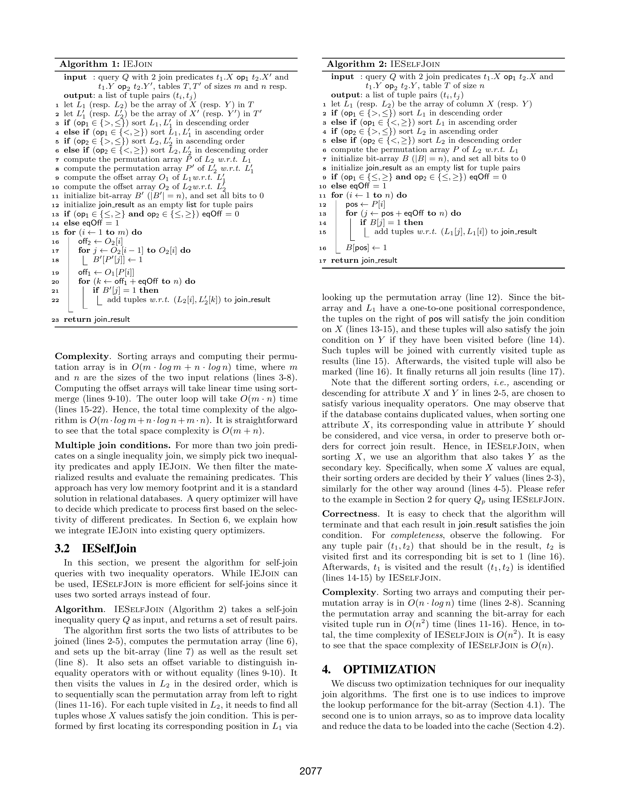
Algorithm 1 (IEJoin) and Algorithm 2 (IESelfJoin) from Khayyat et al. The key difference: IESelfJoin operates on a single table and uses two sorted arrays instead of four, with a Boolean flag to prevent self-matches.

IESelfJoin — Single Table

The simpler case, used when joining a table with itself:

def ie_self_join(
    tuples: list,
    attr1: str,        # first join attribute (e.g., "time")
    attr2: str,        # second join attribute (e.g., "cost")
    op1: str,          # first operator: ">" or "<"
    op2: str,          # second operator: ">" or "<"
) -> list[tuple]:
    n = len(tuples)
 
    # Phase 1: Sort by each attribute independently
    sorted_by_attr1 = sort(tuples, key=attr1)  # ascending or descending per op1
    sorted_by_attr2 = sort(tuples, key=attr2)
 
    # Phase 2: Build the permutation array
    # For each tuple in sorted_by_attr2 order, find its position in sorted_by_attr1
    permutation = []
    for t in sorted_by_attr2:
        pos = index_of(t, in_array=sorted_by_attr1)
        permutation.append(pos)
 
    # Phase 3: Scan and collect results
    visited = BitArray(n)   # all zeros
    results = []
 
    for i in range(n):
        p = permutation[i]          # this tuple's position in attr1-sorted order
 
        # Find all set bits above position p — each is a match
        for match_pos in visited.set_bits_above(p):
            match_tuple = sorted_by_attr1[match_pos]
            current_tuple = sorted_by_attr2[i]
            # Skip self-matches (a tuple can't join with itself)
            if match_tuple != current_tuple:
                results.append((match_tuple, current_tuple))
 
        visited.set(p)
 
    return results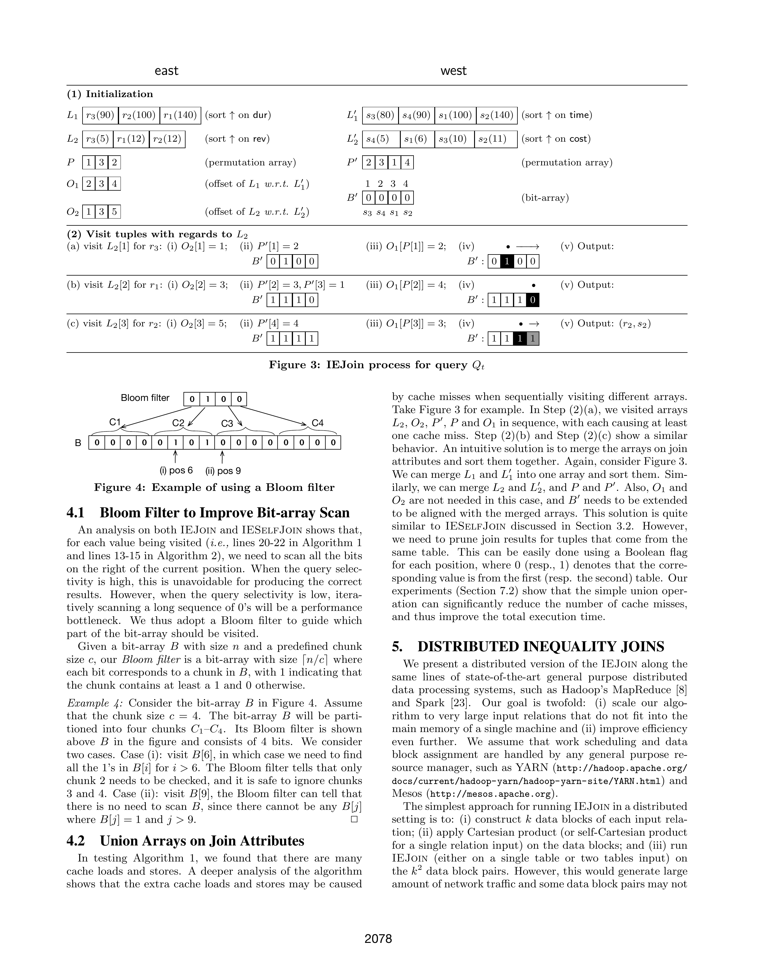

Figure 5 from Khayyat et al.: Permutation array creation for a self-join. After sorting by time (left column) and by cost (right column), the pos column — which records each tuple’s position in the time-sorted order — becomes the permutation array when read in cost-sorted order.

IEJoin — Two Different Tables

When joining two distinct tables (e.g., east and west), the algorithm needs additional data structures to track cross-table positions:

def ie_join(
    left: list,         # e.g., east transactions
    right: list,        # e.g., west transactions
    attr1: str,         # first join attribute (e.g., "dur" / "time")
    attr2: str,         # second join attribute (e.g., "rev" / "cost")
    op1: str,           # ">" or "<"
    op2: str,           # ">" or "<"
) -> list[tuple]:
 
    # Phase 1: Sort each table by each attribute independently
    # This produces FOUR sorted arrays (two per table)
    left_by_attr1  = sort(left,  key=attr1)
    left_by_attr2  = sort(left,  key=attr2)
    right_by_attr1 = sort(right, key=attr1)
    right_by_attr2 = sort(right, key=attr2)
 
    # Phase 2: Permutation arrays — one per table
    # Each maps attr2-sorted positions to attr1-sorted positions
    left_permutation  = [index_of(t, left_by_attr1)  for t in left_by_attr2]
    right_permutation = [index_of(t, right_by_attr1) for t in right_by_attr2]
 
    # Phase 3: Offset arrays — bridge between left and right sorted orders
    # For each left tuple in left_by_attr1, record its relative position
    # among right tuples in right_by_attr1 (and vice versa for attr2).
    # These offsets tell the scan loop WHERE in the other table's bit-array
    # to start looking.
    left_offset  = compute_offsets(left_by_attr1, right_by_attr1)
    right_offset = compute_offsets(left_by_attr2, right_by_attr2)
 
    # Phase 4: Scan — walk through left_by_attr2, mark right_visited
    right_visited = BitArray(len(right))
    results = []
 
    for i in range(len(left)):
        p = left_permutation[i]
 
        # Use offset arrays to find the range of right-side positions
        # that could satisfy the first condition
        start = left_offset[p]
 
        # Mark the corresponding right-side position
        right_p = right_permutation[...]  # determined by offset lookup
        right_visited.set(right_p)
 
        # Scan right_visited for set bits in the valid range
        for match_pos in right_visited.set_bits_in_range(start, ...):
            results.append((left_by_attr2[i], right_by_attr1[match_pos]))
 
    return results

The two-table version is more complex because the offset arrays must bridge two independent sort orders across two different tables. The self-join version above captures the essential algorithm more clearly — start there if the two-table version feels opaque.

Optimizations

Bloom Filter on the Bit-Array

The inner loop scans the visited bit-array to find set bits. When selectivity is low (few matches), most of the scan traverses long runs of zeros — wasted work.

The optimization: partition the bit-array into fixed-size chunks of c bits. Maintain a Bloom filter (a compact probabilistic data structure that answers “is this element in the set?” with possible false positives but no false negatives) — here implemented as a second bit-array of size $⌈ n / c ⌉$ where each bit indicates whether the corresponding chunk contains at least one set bit. Before scanning a chunk, check the Bloom filter — if the chunk bit is 0, skip the entire chunk.

CHUNK_SIZE = 1024  # bits — optimal for L1 cache ≈ 256KB
 
chunk_has_bits = BitArray(ceil(n / CHUNK_SIZE))  # the "Bloom filter"
 
def mark_visited(pos):
    visited.set(pos)
    chunk_has_bits.set(pos // CHUNK_SIZE)
 
def scan_above(pos):
    start_chunk = pos // CHUNK_SIZE
    for chunk_idx in range(start_chunk, num_chunks):
        if not chunk_has_bits.get(chunk_idx):
            continue  # skip entire chunk — no set bits here
        # Only scan within this chunk
        for bit in visited.set_bits_in_chunk(chunk_idx):
            if bit > pos:
                yield bit

The paper found optimal chunk size to be 1,024 bits, achieving a 3x speedup over unchunked scanning. Too-small chunks add overhead; too-large chunks (16K+) don’t filter enough.

Union Arrays for Cache Locality

The original algorithm visits sorted_by_attr2, right_offset, permutation, and left_offset in sequence for each iteration, causing cache misses as it jumps between data structures. The optimization merges related arrays into a single contiguous structure so that all data needed per iteration sits in adjacent memory:

# Before: four separate arrays, four cache lines per iteration
sorted_by_attr2[i]    # cache line A
right_offset[i]       # cache line B (likely different)
permutation[i]        # cache line C
left_offset[p]        # cache line D
 
# After: one struct array, one cache line per iteration
unified[i] = (attr2_value, offset, permutation_pos)

This reduced L1 data cache loads by 2.7x and total execution time by 2.6x in the paper’s benchmarks (10M rows, Events dataset).

Complexity Analysis

	Time	Space
IEJoin (two tables)	$O (m \cdot lo g m + n \cdot lo g n + m \cdot n)$	$O (m + n)$
IESelfJoin	$O (n \cdot lo g n + n^{2})$	$O (n)$

The $m \cdot n$ (or $n^{2}$ ) term comes from the worst case where the outer loop visits every element and the inner scan touches every bit. In practice, with the Bloom filter optimization and when selectivity is moderate, the bit-array scan is much faster.

The space complexity is $O (m + n)$ — just the sorted arrays, permutation arrays, and bit-array. This is a major advantage over index-based approaches (B+-tree, GiST) which require $O (n)$ space per index per attribute.

Experimental Results (from the paper)

On single-node benchmarks (PostgreSQL v9.4):

PG-IEJoin vs. PG-Original: 1–3 orders of magnitude faster for all query types and input sizes (10K–100K rows)
PG-IEJoin vs. PG-BTree/GiST: More than one order of magnitude faster. IEJoin was faster than the index build time alone for BTree
Memory: 150MB for a 200K-row join (vs. MonetDB needing 419GB for the same)

On distributed benchmarks (Spark SQL, 6 nodes):

Spark SQL-IEJoin vs. Spark SQL default: At least one order of magnitude faster
Global sorting improved distributed IEJoin by 2.4–2.9x by filtering out non-intersecting block pairs

Connection to ASOF Join

IEJoin handles the general case: find all pairs satisfying inequality conditions. ASOF Join is a specialization that needs only the best match per left row. This specialization enables much simpler algorithms:

	IEJoin	ASOF Join
Output	All matching pairs	One match per left row
Conditions	Two inequality predicates	One inequality + one equality
Algorithm	Permutation array + bit-array	Two-pointer merge
Time	$O (n lo g n + output)$	$O (n lo g n)$
Best implementation	Bit-array scanning	Sort-merge with monotonic pointers

When a system needs general inequality join support (e.g., range joins, interval overlap queries), IEJoin is the right tool. When the query is specifically “find the most recent match,” the sort-merge ASOF join is simpler and faster.

Edmondo's Vault

Explorer

IEJoin Algorithm

IEJoin Algorithm

The Problem

Core Insight

Worked Example: Self-Join (IESelfJoin)

Input Data

Step 1 — Sort and Build Data Structures

Step 2 — The Main Loop

Why This Works

What About the Inner Loop?

Algorithm Pseudocode

IESelfJoin — Single Table

IEJoin — Two Different Tables

Optimizations

Bloom Filter on the Bit-Array

Union Arrays for Cache Locality

Complexity Analysis

Experimental Results (from the paper)

Connection to ASOF Join

See also

Graph View

Table of Contents

Backlinks