Lagrange Multipliers

The problem: optimization with constraints

In unconstrained optimization (see Critical Points and the Hessian), we find the extrema of a function $f(x,y)$ by setting $\nabla f=0$ (see Directional Derivatives and the Gradient for the gradient) and solving. This works because at an interior extremum, the directional derivative is zero in every direction, which forces the gradient to vanish.

But many real problems come with constraints --- restrictions that confine the domain to a specific curve or surface. For example:

• Minimize cost $f(x,y)$ subject to a production requirement $g(x,y)=c$.
• Find the closest point on a curve to the origin: minimize $f(x,y)=x^2+y^2$ subject to the curve equation $g(x,y)=c$.
• Maximize area subject to a fixed perimeter.

In these problems, we cannot simply set $\nabla f=0$. The extremum may occur at a point where $\nabla f\ne 0$ --- the gradient does not vanish, but the extremum exists because we are restricted to the constraint curve $g(x,y)=c$. We need a different approach.

The method of Lagrange multipliers, developed by Joseph-Louis Lagrange in 1788 in his Mecanique Analytique, provides that approach. There are two ways to derive it: a geometric argument based on tangent level curves, and an analytic argument based on the chain rule. Both lead to the same condition.

Path 1 --- Geometric derivation (tangent level curves)

Tangency from first principles

Before we can state the geometric argument, we need a precise definition of what it means for two curves to be tangent.

A smooth curve in ${\mathbb{R}}^2$ is a set of points that can be described by a parametrization --- a vector-valued function $\mathbf{r}(t)=(x(t),y(t))$ where $x(t)$ and $y(t)$ are differentiable functions of a parameter $t$ (see Arc-Length Parametrization for parametrizations and the role of arc length). The tangent vector at a point $P=\mathbf{r}(t_0)$ is

$${\mathbf{r}}^{\prime }(t_0)=\left(\frac{dx}{dt}(t_0),\frac{dy}{dt}(t_0)\right).$$

This vector points in the instantaneous direction of motion along the curve. The tangent line at $P$ is the unique line through $P$ in the direction of ${\mathbf{r}}^{\prime }(t_0)$:

$$\ell (s)=P+s{\mathbf{r}}^{\prime }(t_0),s\in \mathbb{R}.$$

Now consider two smooth curves ${\mathcal{C}}_1$ and ${\mathcal{C}}_2$ that pass through the same point $P$. We say the curves are tangent at $P$ when they share the same tangent line at $P$ --- equivalently, their tangent vectors at $P$ are parallel (one is a scalar multiple of the other).

Tangent vs. intersecting

Two curves can intersect at a point without being tangent --- they cross at an angle, like an X. Tangency means they touch and locally point in the same direction, like two roads merging smoothly.

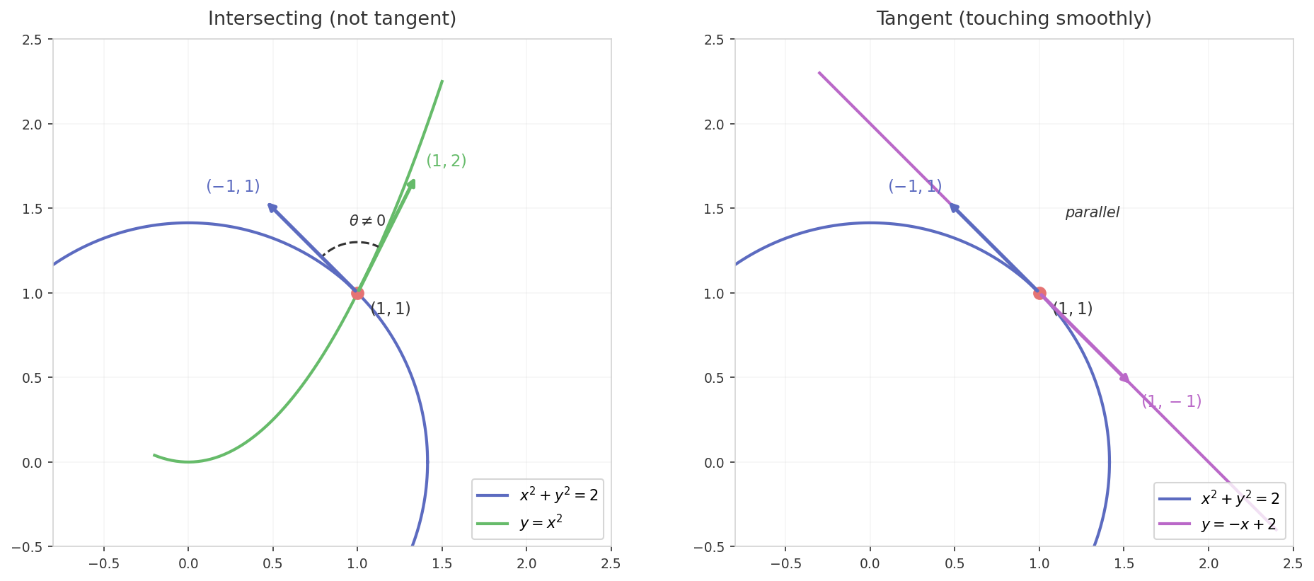
Concrete example. The diagram above shows the circle $x^2+y^2=2$ meeting two different curves at the same point $(1,1)$. Left: the parabola $y=x^2$ intersects the circle --- the tangent vectors point in different directions ($\theta \ne 0$). Right: the line $y=-x+2$ is tangent to the circle --- the tangent vectors are parallel.

Let’s verify this with computation. Parametrize the circle as ${\mathbf{r}}_1(t)=(\sqrt{2}\cos t,\sqrt{2}\sin t)$ and the parabola as ${\mathbf{r}}_2(t)=(t,t^2)$.

Tangent vector of the circle at $(1,1)$. The point $(1,1)=(\sqrt{2}\cos \frac{\pi }{4},\sqrt{2}\sin \frac{\pi }{4})$ corresponds to $t=\frac{\pi }{4}$:

$${\mathbf{r}}_1^{\prime }(t)=(-\sqrt{2}\sin t,\sqrt{2}\cos t),{\mathbf{r}}_1^{\prime }\left(\frac{\pi }{4}\right)=(-1,1).$$

Tangent vector of the parabola at $(1,1)$. The point $(1,1)$ corresponds to $t=1$:

$${\mathbf{r}}_2^{\prime }(t)=(1,2t),{\mathbf{r}}_2^{\prime }(1)=(1,2).$$

Are $(-1,1)$ and $(1,2)$ parallel? Two vectors are parallel if one is a scalar multiple of the other: $(-1,1)=\lambda (1,2)$ requires $\lambda =-1$ from the first component and $\lambda =\frac{1}{2}$ from the second. These are inconsistent, so the vectors are not parallel. The circle and parabola intersect at $(1,1)$ but are not tangent there --- they cross at an angle.

For a tangent point, we would need a curve whose tangent vector at the intersection is a scalar multiple of $(-1,1)$. The line $y=-x+2$ passes through $(1,1)$ with direction vector $(1,-1)=-1\cdot (-1,1)$, so this line is tangent to the circle at $(1,1)$ --- as shown in the right panel.

The level curve picture

Now apply the tangency concept to constrained optimization. Consider the function $f(x,y)$ and the constraint $g(x,y)=c$.

A level curve (also called a contour) of $f$ is the set of all points where $f$ takes a specific constant value: $\{(x,y):f(x,y)=k\}$ (see Directional Derivatives and the Gradient for the full treatment of level curves and their relationship to the gradient). As $k$ increases, the level curves of $f$ sweep across the plane. Think of a topographic map: each contour line is a level curve of the elevation function, and higher contour values correspond to higher ground.

Walking along the constraint

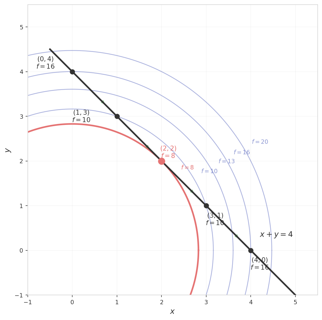
Imagine drawing the constraint curve $g(x,y)=c$ on top of these level curves. The diagram above shows this for $f(x,y)=x^2+y^2$ (whose level curves are circles centered at the origin) with the constraint $x+y=4$ (the dark line).

Now walk along the constraint and track how $f$ changes:

Position on constraint	$f=x^2+y^2$	What happens
$(0,4)$	$16$	Starting point --- far from the origin
$(1,3)$	$10$	Crossed from the $f=16$ circle inward to $f=10$ --- $f$ decreased, keep going
$(2,2)$	$8$	Reached the $f=8$ circle --- the constraint just touches this circle
$(3,1)$	$10$	Crossed back outward to $f=10$ --- $f$ increased, we passed the minimum
$(4,0)$	$16$	Back to $f=16$ --- symmetric with the start

At $(1,3)$, the level curve $f=10$ crosses the constraint line --- the curves intersect transversally. You can keep walking and reach a smaller value of $f$. This is not the minimum.

At $(2,2)$, the level curve $f=8$ touches the constraint without crossing it. Walking in either direction takes you to larger circles ($f>8$). This is the constrained minimum --- and the level curve is tangent to the constraint here.

Core geometric insight

Constrained extrema of $f$ on the curve $g=c$ occur where a level curve of $f$ is tangent to the constraint curve $g=c$.

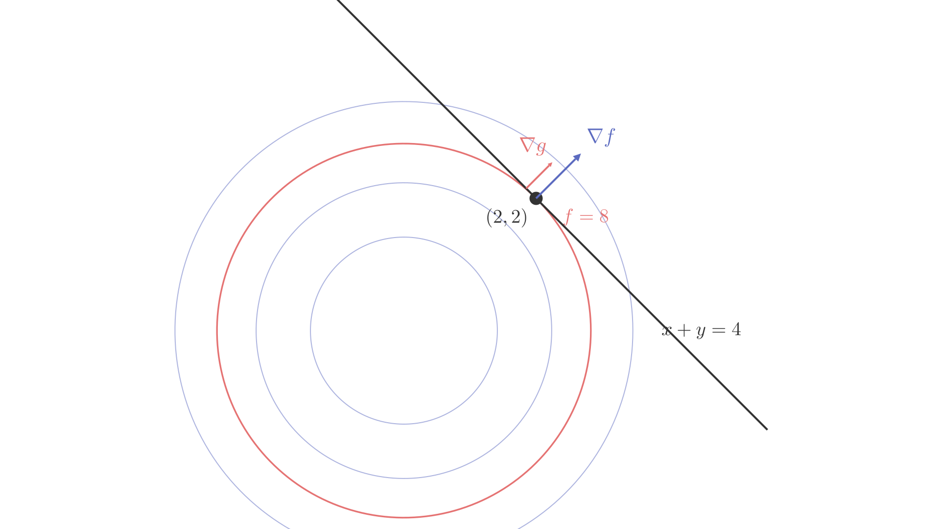
The diagram above zooms in on the tangent point. The parallel gradient arrows $\nabla f$ (blue) and $\nabla g$ (red) at $(2,2)$ confirm the Lagrange condition $\nabla f=\lambda \nabla g$ --- the gradients point in the same direction because the curves are tangent.

Tangency implies parallel normals

At a tangent point, the level curve of $f$ and the constraint curve $g=c$ share the same tangent line. A normal vector to a curve at a point is any vector perpendicular to the tangent line at that point.

Since the two curves share the same tangent line, any vector perpendicular to that tangent line is simultaneously normal to both curves. In particular, the normal vectors of the two curves must point along the same line --- they are parallel (one is a scalar multiple of the other).

The gradient is the normal

From Directional Derivatives and the Gradient, the gradient $\nabla f$ at a point is perpendicular to the level curve of $f$ through that point. Similarly, $\nabla g$ is perpendicular to the level curve of $g$ --- and the constraint $g(x,y)=c$ is itself a level curve of $g$.

So:

• The normal to the level curve of $f$ at the tangent point is $\nabla f$.
• The normal to the constraint curve $g=c$ at the tangent point is $\nabla g$.

The condition “normals are parallel” becomes:

$$\boxed{\nabla f=\lambda \nabla g}$$

for some scalar $\lambda$, called the Lagrange multiplier.

Path 2 --- Analytic derivation ($df/ds=0$ on the constraint)

Restriction to the constraint

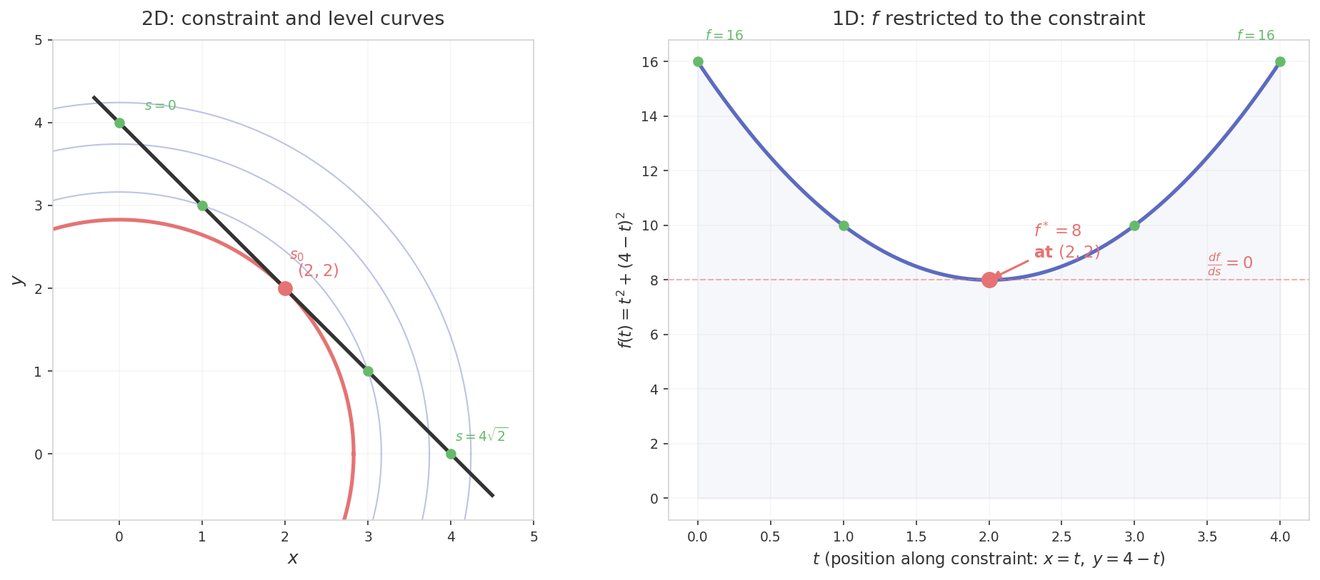
The key idea of Path 2 is to forget the 2D plane entirely and view $f$ as a function of a single variable: position along the constraint. The diagram above shows both views side by side. Left: the familiar 2D picture with level curves and constraint. Right: the same information collapsed to one dimension --- $f$ plotted against position $t$ along the constraint line $x+y=4$ (where $x=t$, $y=4-t$).

The 1D picture makes the extremum obvious: $f(t)=t^2+(4-t{)}^2$ is a parabola with a minimum at $t=2$. At the minimum, the curve is flat --- $\frac{df}{ds}=0$. This is just single-variable calculus.

To make this precise: parametrize the constraint by arc length $s$. Then $f$ becomes a function of the single variable $s$: the value of $f$ at whatever point on the constraint corresponds to position $s$.

If $f$ has a constrained maximum or minimum at a point $P$ on the constraint, then $f$-as-a-function-of-$s$ has a local maximum or minimum at the corresponding $s_0$. By single-variable calculus, a necessary condition for a local extremum is

$$\frac{df}{ds}{|}_{s=s_0}=0.$$

Clarification

$\frac{df}{ds}=0$ does not mean $f$ is constant on the constraint. It means that at this specific point, $f$ (viewed as a function of position along the constraint) has a local extremum. Like a hilltop on a mountain trail: the trail keeps going, but the elevation momentarily stops changing. Before and after this point, $f$ may well be increasing or decreasing along the constraint.

Chain rule

Let $\mathbf{u}$ be the unit tangent vector to the constraint curve at $P$. The condition ”$f$ has a constrained extremum at $P$” can be rephrased as: the derivative of $f$ along any tangent vector of the constraint $g=c$ must be zero at $P$. This is exactly the single-variable extremum condition applied to the restriction of $f$ to the constraint.

By the chain rule:

$$\frac{df}{ds}=\nabla f\cdot \mathbf{u}.$$

At the constrained extremum, $\frac{df}{ds}=0$, so

$$\nabla f\cdot \mathbf{u}=0.$$

This means $\nabla f$ is perpendicular to $\mathbf{u}$. But $\nabla g$ is also perpendicular to $\mathbf{u}$, because $\nabla g$ is perpendicular to the level curves of $g$ (and the constraint $g=c$ is a level curve of $g$).

In ${\mathbb{R}}^2$, there is only one independent direction perpendicular to a given line direction. Since both $\nabla f$ and $\nabla g$ are perpendicular to the same tangent direction $\mathbf{u}$, they must be parallel:

$$\nabla f=\lambda \nabla g.$$

Both paths agree

Path 1 (tangent level curves) and Path 2 ($df/ds=0$) produce the same necessary condition: $\nabla f=\lambda \nabla g$. The geometric argument gives visual intuition --- constrained extrema occur where level curves kiss the constraint. The analytic argument gives a rigorous chain-rule proof. Together, they reinforce the result from complementary perspectives.

Completing the solution

The system of equations

For a function $f(x,y)$ subject to a single constraint $g(x,y)=c$, the condition $\nabla f=\lambda \nabla g$ expands to two scalar equations:

$$\frac{\partial f}{\partial x}=\lambda \frac{\partial g}{\partial x},\frac{\partial f}{\partial y}=\lambda \frac{\partial g}{\partial y}.$$

Adding the constraint itself gives a third equation:

$$g(x,y)=c.$$

This is a system of three equations in three unknowns: $x$, $y$, and $\lambda$. Solving this system yields the candidate points for constrained extrema.

Higher dimensions

For $f(x_1,\dots ,x_n)$ subject to $g(x_1,\dots ,x_n)=c$, the condition $\nabla f=\lambda \nabla g$ gives $n$ scalar equations. Together with the constraint, that is $n+1$ equations in $n+1$ unknowns ($x_1,\dots ,x_n,\lambda$). For $m$ constraints $g_1=c_1,\dots ,g_m=c_m$, the condition becomes $\nabla f={\lambda }_1\nabla g_1+\cdots +{\lambda }_m\nabla g_m$, giving $n+m$ equations in $n+m$ unknowns.

What $\lambda$ means: the shadow price

The multiplier $\lambda$ is not just an algebraic device for solving the system --- it has a direct interpretation. Let $f^{\ast }(c)$ denote the optimal value of $f$ as a function of the constraint level $c$. Then

$$\lambda =\frac{d{f}^{\ast }}{dc}.$$

That is, $\lambda$ measures how much the optimum improves (or worsens) per unit relaxation of the constraint. In economics, this is called the shadow price --- the marginal value of relaxing the constraint by one unit. A large $|\lambda |$ means the constraint is binding tightly: loosening it even slightly would significantly change the optimal value. A small $|\lambda |$ means the constraint is nearly slack.

Worked example

Problem. Minimize $f(x,y)=x^2+y^2$ subject to $g(x,y)=x+y=4$.

Geometrically: find the point on the line $x+y=4$ that is closest to the origin (since $x^2+y^2$ is the squared distance to the origin).

Step 1: Compute the gradients.

$$\nabla f=(2x,2y),\nabla g=(1,1).$$

Step 2: Set up $\nabla f=\lambda \nabla g$.

$$2x=\lambda \cdot 1,2y=\lambda \cdot 1.$$

From the first equation, $\lambda =2x$. From the second, $\lambda =2y$. Therefore $2x=2y$, so $x=y$.

Step 3: Apply the constraint.

$$x+y=4⟹2x=4⟹x=2,y=2.$$

Step 4: Compute $\lambda$ and $f^{\ast }$.

$$\lambda =2x=4,f^{\ast }=f(2,2)=4+4=8.$$

The closest point on the line $x+y=4$ to the origin is $(2,2)$, at squared distance $8$.

Step 5: Verify the shadow price interpretation.

Change the constraint to $x+y=4.1$ and re-solve. The same argument gives $x=y=2.05$, so

$$f_{\text{new}}^{\ast }=(2.05{)}^2+(2.05{)}^2=2\times 4.2025=\mathrm{8.405.}$$

The change in optimal value is

$$\Delta f^{\ast }=8.405-8=0.405\approx \lambda \times \Delta c=4\times 0.1=\mathrm{0.4.}$$

The small discrepancy ($0.405$ vs. $0.4$) is the second-order error --- $\lambda =\frac{d{f}^{\ast }}{dc}$ is exact only in the limit $\Delta c\to 0$. But even for a finite step of $\Delta c=0.1$, the approximation $\Delta f^{\ast }\approx \lambda \Delta c$ is very close, confirming the interpretation.

See also

• Directional Derivatives and the Gradient --- the gradient-perpendicular-to-level-curves result that underpins both derivation paths
• Critical Points and the Hessian --- unconstrained optimization and the second-derivative test; Lagrange multipliers handle the constrained case
• Arc-Length Parametrization --- parametrization by arc length used in Path 2 to restrict $f$ to the constraint curve