Distributed Training for Embedding-Heavy Recommenders

Distributed training for embedding-heavy recommenders splits batch work and model storage across GPUs because the embedding tables, optimizer bookkeeping, or target throughput exceed one device. Multiple Embedding Tables in Recommender Rankers explains the candidate-row lookup fan-out that this note distributes across ranks.

A rank is one participating training process, usually bound to one GPU. A node is one machine that hosts several GPUs. A shard is the slice of model data owned by one rank or group of ranks, such as a range of embedding rows or a slice of weights. A replica is one complete copy of the model, even if that copy is internally sharded.

Why The Shuffle Exists

The shuffle is necessary because the rank that owns a training example is often not the rank that owns every embedding row referenced by that example.

Suppose rank 0 receives this local batch:

rank 0 local batch:
  row A: user_42, pin_77, board_789
  row B: user_99, pin_12, board_555

The embedding tables are sharded by owner:

rank 0 owns user rows
rank 1 owns pin rows
rank 2 owns board rows

Rank 0 has the examples, but it cannot assemble the model input locally. It has user rows, but it does not have the Pin or board vectors. The framework routes lookup requests to the row owners:

rank 0 -> rank 1: please return pin_77, pin_12
rank 0 -> rank 2: please return board_789, board_555
 
rank 1 -> rank 0: vector(pin_77), vector(pin_12)
rank 2 -> rank 0: vector(board_789), vector(board_555)

That routing is the distributed embedding lookup shuffle. With many ranks, every rank can be both a batch owner asking for remote rows and a row owner answering other ranks.

One Training Step

This diagram shows the same ownership problem at GPU scale. Each rank processes local examples, but the ids in those examples may refer to embedding rows owned by other ranks.

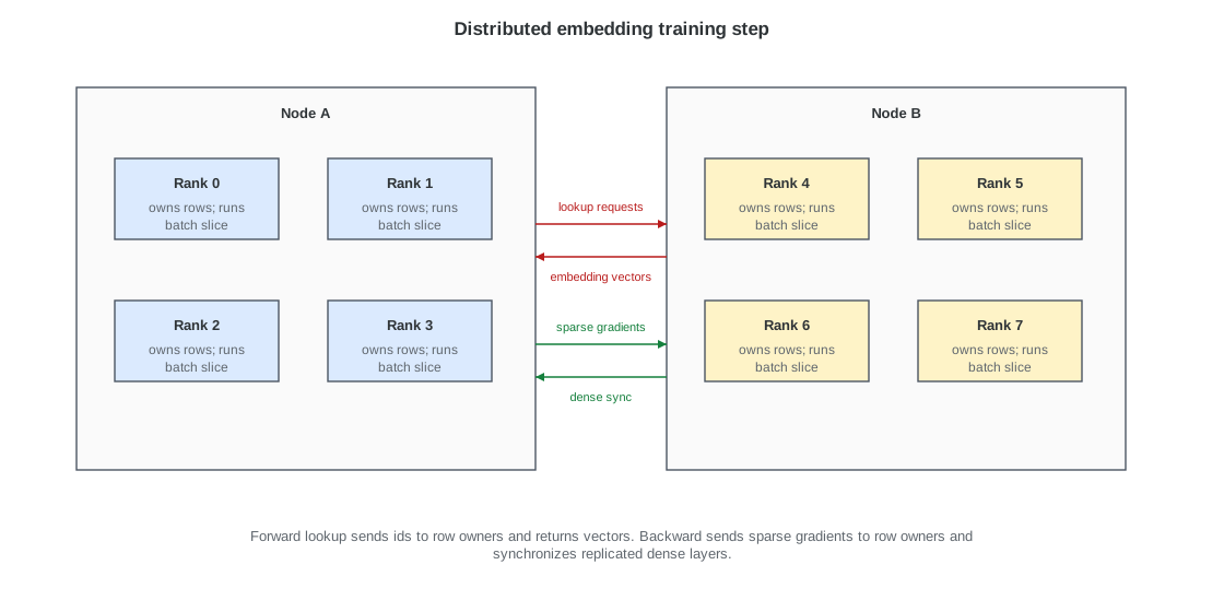
One training step has this lifecycle:

1. Local batch input. Each rank receives labeled candidate rows.
2. Lookup routing. The framework maps each id to the rank that owns the embedding row.
3. Vector return. Row owners return embedding vectors to the ranks assembling candidate-row tensors.
4. Local model compute. Each rank runs the interaction layers for its local batch slice.
5. Sparse-gradient return. Backpropagation produces gradients for touched embedding rows; those gradients return to the row owners.
6. Dense-gradient synchronization. If dense layers are replicated, ranks combine dense gradients so replicas apply aligned updates.
7. Optimizer update. Embedding owners update their local rows. Dense replicas update from synchronized gradients.

The expensive payload is not the raw id. The expensive payload is the returned vector and the gradient information tied to that vector.

Code-Like Routing Sketch

The training framework hides most of this routing, but the ownership logic is roughly:

local_ids = {
    "pin": [77, 12],
    "board": [789, 555],
}
 
requests_by_owner = {
    rank_for("pin", 77): [("pin", 77)],
    rank_for("pin", 12): [("pin", 12)],
    rank_for("board", 789): [("board", 789)],
    rank_for("board", 555): [("board", 555)],
}
 
remote_vectors = all_to_all_lookup(requests_by_owner)
candidate_tensor = assemble(local_dense_features, remote_vectors)
loss = model(candidate_tensor, labels)
loss.backward()
send_sparse_gradients_to_row_owners()

The point is not the Python API. The point is the data dependency: a rank cannot run the next layer until it has the vectors for the ids in its local candidate rows.

Sharding Choices

Table-wise sharding places whole embedding tables on different ranks. It is simple, but one rank can become overloaded if it owns a large or hot table.

Row-wise sharding splits rows of one table across ranks. It balances memory for a large table, but lookup traffic fans out whenever a batch references rows owned by many ranks.

Hash partitioning assigns ids to shards through a hash function. It avoids storing a placement record for every id, but it does not remove hot-key or hot-feature skew by itself.

Column-wise sharding splits embedding dimensions across ranks. It can reduce per-rank memory for wide embeddings, but consumers need all dimension slices before the next layer can see the full vector.

TorchRec uses planners and sharding abstractions so model authors can express embedding tables while the framework maps tables and rows onto ranks. The placement still defines the communication shape.

Why Multi-Node Is Different

Within one node, GPUs often communicate through local high-bandwidth interconnects. Across nodes, traffic crosses network devices and distributed communication libraries. The same logical lookup shuffle becomes more expensive when row owners live on other machines.

For an embedding-heavy model, global sharding can increase the number of possible remote owners for each lookup. Rank 0 on node A may need vectors from nodes B, C, and D in the same forward pass. The model fits, but the step waits on cross-node data movement.

Profiling Signals

SM efficiency means the fraction of streaming-multiprocessor cycles retiring useful GPU math. A communication-bound step can show high GPU utilization while SM efficiency stays low because communication kernels are active but matrix math is not progressing.

Read profiler symptoms against the training-step lifecycle:

Signal	Stage implicated	Diagnosis
High GPU utilization with low SM efficiency	lookup exchange or synchronization	GPUs are busy moving or waiting on tensors
Long NCCL send/recv kernels	all-to-all or all-reduce	communication dominates the trace
Forward pass grows when adding nodes	vector return	embedding vectors cross slower inter-node links
Throughput scales sublinearly	any gated stage	extra GPUs wait for communication, input, or load-skewed shards

The Pinterest article reports this failure mode: the model fit through TorchRec sharding, but multi-node forward time grew because distributed embedding lookup communication dominated.

Sources

• Pinterest Engineering - Achieving Near-Linear Training Scalability for Pinterest’s Foundation Models
• TorchRec documentation
• PyTorch distributed overview

See also

• Embedding-Heavy Models
• Multiple Embedding Tables in Recommender Rankers
• GPU Collective Communication
• Training Scalability for Distributed ML
• 2D Parallelism for Recommendation Model Training