Cloud instance selection by workload shape is the discipline of matching a workload’s first scarce resource to the machine family that exposes that resource at low cost with the right failure contract. A large production estate does not spend money on one generic kind of “compute.” It spends money on request serving, ranking, feature retrieval, storage engines, logs, data processing, object storage, data transfer, and shared platforms. Each has a different unit of work and a different failure mode.
Ask the node-choice question in operational terms: what does this node do, what resource saturates first, and what business unit does that resource produce?
Workload Map
Read each row as a translation path: start with the workload shape, identify the first resource that becomes scarce, then inspect the cost object that exposes the bill.
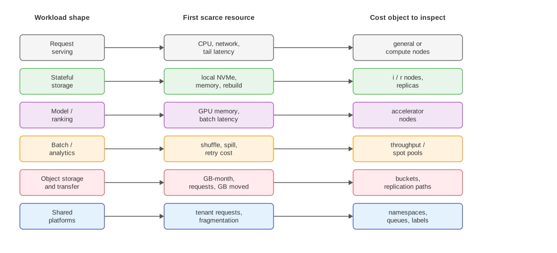
The same product can need several machine shapes at once. Request serving, stateful storage, model inference, analytics, object storage, and shared schedulers expose different bottlenecks, so one “large instance” mental model is too coarse.
Request-serving nodes handle live user or API traffic. Their first constraints are often p95/p99 latency, CPU headroom, network fanout, connection pools, and overload behavior. General-purpose or compute-optimized nodes fit when the workload is stateless and can scale by adding nodes.
Stateful storage nodes hold shard-local data: key-value state, search segments, stream logs, caches, or database replicas. Their first constraints are memory, local NVMe latency, write amplification, replication bandwidth, and rebuild time. Storage-optimized nodes are not “big compute”; they are local-state machines.
Model and ranking nodes score items, requests, documents, images, ads, or other candidates. Their first constraints are model memory, accelerator utilization, batch latency, CPU preprocessing, and queueing. GPU or other accelerator nodes fit when the model’s dense tensor work can keep the accelerator busy.
Batch and analytics nodes process logs, train features, compact data, backfill tables, or run queries. Their first constraints are throughput, shuffle/network bandwidth, object-store reads, spill behavior, retry cost, and deadline. The best node may be cheaper retryable capacity, not the lowest-latency machine.
Shared platform nodes run other people’s workloads through Kubernetes, batch schedulers, workflow engines, or managed platforms. The instance type describes the host, but the spending cause lives in tenant requests, quotas, pod shapes, queue policy, and attribution. The host instance type by itself hides the real owner.
Lessons From A Real Production Estate
A production cost report becomes useful after translating names into workload mechanics. These are the reusable lessons.
| Observation | General lesson | Better question |
|---|---|---|
| Small storage-optimized nodes can dominate instance-hours | Always-on stateful fleets accumulate cost through volume and uptime, not exotic hardware | Which services need local NVMe, and can they rebuild or replicate without violating recovery targets? |
| GPU nodes are expensive but not self-explanatory | Accelerator spend often means model inference, ranking, embedding, or image/video work | What is cost per useful prediction within the latency target? |
| Large CPU or memory nodes often sit near ML systems | Model serving includes feature fetch, preprocessing, calibration, policy, merging, and logging | Is CPU/network feeding the accelerator, or duplicating avoidable work? |
| Object storage and data transfer can rival EC2 line items | Instance reports miss data-lake, logs, replication, and egress costs | Which datasets, buckets, or streams create the storage and transfer bill? |
| Shared schedulers hide tenants | A host fleet can be “Kubernetes” while the cause is a specific product, job, or namespace | Can cost be attributed to pod requests, job labels, queue, or tenant? |
| Organization names are accounting views | The same technical system may be split across product, platform, and data owners | Which boundary is being used: org, project, service, platform, tenant, or bucket? |
The practical effect is that “top spender” is not yet an explanation. It is a pointer to a lifecycle stage. A useful analysis names the stage, the saturated resource, the unit of work, and the owner who can change it.
Instance Families As Workload Hints
Cloud instance names are compressed workload hints. In AWS-style names, the family prefix is the first decision signal: g often means GPU, i means storage-optimized with local NVMe, r means memory-optimized, c means compute-optimized, and m means balanced general purpose. The generation and suffix refine the processor, network, storage, or accelerator variant; the size controls how much of that shape is exposed.
The size suffix is not the workload. In these representative AWS 2xlarge examples, the vCPU count stays at 8 while the family changes the memory, local storage, and accelerator ratio. Verify current provider docs before using exact numbers in a capacity plan.
| Family signal | Representative shape | Memory ratio | Extra resource | What the ratio buys |
|---|---|---|---|---|
c compute optimized | c7i.2xlarge: 8 vCPU, 16 GiB | 2 GiB/vCPU | No local instance store | Dense CPU slots for request handlers, rules, lightweight ranking, compression, parsing, and fanout control. |
m general purpose | m7i.2xlarge: 8 vCPU, 32 GiB | 4 GiB/vCPU | No local instance store | More memory headroom for mixed services with caches, sidecars, larger request objects, or runtime overhead. |
r memory optimized | r7i.2xlarge: 8 vCPU, 64 GiB | 8 GiB/vCPU | No local instance store | Larger resident sets for caches, indexes, query state, and services where garbage collection or page cache pressure hurts tail latency. |
i storage optimized | i4i.2xlarge: 8 vCPU, 64 GiB | 8 GiB/vCPU | 1 x 1875 GB local NVMe SSD | Local random I/O and write bandwidth for shards, compaction, brokers, and rebuildable local state. |
g GPU optimized | g6.2xlarge: 8 vCPU, 32 GiB | 4 GiB/vCPU | 1 NVIDIA L4 GPU plus local NVMe SSD | Accelerator memory and tensor throughput for models, with enough CPU and local scratch space to feed the GPU. |
This table reads instance families as workload fit, not as a provider recommendation.
| Workload shape | First bottleneck to test | Typical node family | Why that shape fits |
|---|---|---|---|
| Stateless API or request router | CPU, network, connection count | m or c | Balanced or CPU-heavy nodes keep per-request overhead cheap and support scale-out. |
| Feature retrieval fanout | Network, memory, serialization | m, r, or network-enhanced variants | The service needs many concurrent remote reads and enough memory for caches or decoded feature state. |
| Search or candidate index shard | Memory, local disk, random I/O | r or i | Indexes need hot RAM plus predictable local reads; storage-optimized nodes help when local SSD latency dominates. |
| Key-value store or log-backed local state | Local NVMe, memory, replication bandwidth | i | Local SSD absorbs random reads/writes, compaction, and replica catch-up better than a plain general-purpose node. |
| Neural model inference or ranking | GPU memory, accelerator throughput, batch latency | g, p, inf, or similar accelerator families | Tensor-heavy models become cheaper per prediction when batching keeps the accelerator busy. |
| Lightweight ranking, rules, calibration, allocation | CPU and tail latency | c or m | The bottleneck is branchy CPU work and low-latency execution, not accelerator throughput. |
| Query workers, ETL, compaction, backfills | Disk/network throughput, memory, retry cost | m, r, i, or batch/spot pools | The job can trade latency for throughput, queueing, and cheaper retryable capacity. |
| Shared Kubernetes or scheduler hosts | Pod requests, fragmentation, noisy neighbors | Fleet-standard m, c, r, or g pools | The host shape is a platform decision; the workload decision is tenant resource shape and scheduling policy. |
The table has repeated families because instance family and workload stage answer different questions. The family says which resource ratio the provider sells. The workload stage says what the service does with that ratio. A stateless API tier and a lightweight ranker may both land on c or m, but they should prove different claims.
Stage using c or m | Why the same family can fit | Different metric to inspect |
|---|---|---|
| Stateless request serving | The service spends CPU on parsing, auth, routing, serialization, and network fanout. m fits when memory headroom or sidecars matter; c fits when CPU per request dominates. | Cost per request, p99 latency under load, connection churn, overload behavior. |
| Lightweight ranking, rules, calibration, allocation | The service spends CPU on branch-heavy scoring, joins over small in-memory structures, policy checks, and final ordering. m fits when candidate or feature state expands in memory; c fits when scoring is CPU-bound and cache fit is healthy. | Cost per candidate scored, p99 scoring latency, cache-miss rate, CPU cycles per candidate. |
| Feature retrieval coordinator | The service spends CPU on request construction and serialization but waits on network calls. m or network-enhanced variants fit when concurrency and buffers dominate. | Remote read fanout, in-flight request count, memory per open request, timeout rate. |
Treat “same family” as a hypothesis, not a diagnosis. If two services both use m7i.2xlarge, one may need memory for request buffers while another is using the same family because the fleet has better discounts or capacity there. The workload claim has to name the saturated resource and unit of work.
Why A Storage-Optimized Node Exists
A storage-optimized node exists for services whose working set is too large or too write-heavy to treat disk as a distant detail. An i4i.2xlarge-style machine is small in CPU terms: 8 vCPU and 64 GiB of memory. Its distinguishing resource is a local 1875 GB NVMe SSD attached to the instance. That makes it a storage-ratio choice: the service buys the same vCPU count as a 2xlarge general-purpose node, but with much more memory per vCPU and local disk that can absorb shard-local reads, writes, and compaction.
That shape fits workloads such as:
| Workload | Why local NVMe helps | What to verify |
|---|---|---|
| LSM-tree key-value store | Compaction and random reads hit local disk again and again | Write amplification, compaction backlog, p99 read latency |
| Search index shard | Hot postings or segment files can stay local to the serving node | Cache hit rate, shard size, rebuild time |
| Stream broker | Sequential writes and catch-up reads are local and high-throughput | Replication lag, disk utilization, recovery behavior |
| Feature store cache | Misses and refreshes can land in local persistent cache | Hit rate, eviction pressure, stale-data tolerance |
The risk is failure semantics. Local NVMe is tied to the instance. If the node dies, the data on that disk should be treated as gone unless the service replicates it elsewhere. A storage-optimized node is appropriate when the system already has replication, rebuild, or rehydration mechanics.
Why A GPU Node Exists
A GPU node exists when the model’s useful work is dominated by dense tensor operations that can be batched. The accelerator is expensive, so the scheduling problem is to keep it fed without violating request latency. The CPU, memory, network, and preprocessing path are supporting resources; if any of them starve the GPU, the expensive part sits idle.
For online inference, the practical controls are:
| Control | What it changes | Failure mode |
|---|---|---|
| Batch size | More requests per GPU pass improves throughput | Requests wait too long for the batch or finish behind a large batch |
| Model precision or quantization | Smaller tensors reduce memory and bandwidth | Quality or calibration may shift |
| Candidate count | Fewer items require fewer scores | Recall, marketplace pressure, or result quality may drop |
| Feature payload size | Smaller inputs reduce network and serialization cost | Model may lose predictive signal |
| CPU preprocessing | Faster tokenization, normalization, or feature packing feeds the GPU | GPU utilization looks low even though demand is high |
GPU choice should be made from cost per useful prediction within the latency target. Hourly price alone is misleading: a larger GPU node can be cheaper if it serves enough more predictions per hour, while a smaller GPU can be better if the model fits with headroom and traffic is latency-sensitive.
Why Large CPU Or Network Nodes Still Show Up Around Accelerators
Accelerated systems include work around model execution. A production path may have CPU-heavy or network-heavy nodes near the GPU fleet because they build requests, fetch features, apply rules, merge model outputs, enforce policy, compute utility, or write logs. These nodes can look surprising in a cost report because they sit near a model-serving path but do not have GPUs.
Common reasons:
| Surrounding component | Resource pressure | Why it may not belong on the GPU node |
|---|---|---|
| Feature hydrator | Network fanout, memory, serialization | It waits on remote data and prepares inputs. |
| Request batcher | Queues, timers, connection pools | It manages latency/throughput tradeoffs rather than tensors. |
| Calibration or policy layer | Branchy CPU logic | GPU kernels are inefficient for small conditional logic. |
| Result merger | CPU and memory bandwidth | It combines scores with candidate metadata and business rules. |
| Logging sidecar or worker | Network and disk throughput | It should not block the request path or steal accelerator headroom. |
Why Non-Instance Costs Belong In The Same Analysis
Instance spend is one layer of the workload. Data-heavy systems often spend a large amount on object storage, request charges, data transfer, managed databases, monitoring, logs, and platform fees. A compute-only report can make a system look efficient while its data footprint is growing faster than its traffic.
Use this decomposition when a service’s instance choice looks reasonable but total cost still grows:
| Cost layer | Mechanism | Unit to inspect |
|---|---|---|
| Object storage | Logs, tables, model artifacts, index snapshots, backups | GB-month, object count, read/write requests |
| Data transfer | Cross-AZ replication, cross-region copy, egress, fanout | GB transferred by source/destination |
| Managed platform | Shared database, stream, cache, scheduler, or observability backend | Tenant, namespace, topic, bucket, table, queue |
| Commitments and reservations | Savings plans, reserved capacity, unused capacity | Covered hours, idle reserved hours, on-demand spill |
| Shared compute | Kubernetes or batch hosts | Pod request-hours, job runtime, queue, namespace |
This is why cost attribution must preserve both the technical boundary and the accounting boundary. The platform says where the bill landed; the workload shape says who can change the bill.
Decision Procedure
Use this procedure before blessing or challenging a node choice.
- Name the lifecycle stage. Is the node serving requests, retrieving candidates, fetching features, scoring models, running analytics, storing local state, transferring data, or hosting shared tenants?
- Name the first saturated resource. Use p95/p99 CPU, memory, network, disk I/O, accelerator utilization, queueing delay, storage growth, and error rates. Average CPU is not enough.
- Check the unit of work. Measure cost per request, prediction, candidate scored, feature row fetched, query served, GB processed, log event written, or tenant request-hour.
- Separate fit from fleet policy. A workload may fit a niche instance while still being a bad fleet choice because capacity is scarce, discounts do not cover it, or operational support is immature. See Compute Fleet Strategy.
- Benchmark the nearest boring alternative. Compare the chosen type against the blessed general-purpose, compute-optimized, memory-optimized, storage-optimized, or accelerator fallback.
- State the failure contract. For local NVMe, say how data is rebuilt. For GPU, say what happens when the model does not fit or the batch queue grows. For memory-heavy services, say what happens at OOM. For network-heavy services, say what happens at fanout timeout. For shared schedulers, say what happens when tenants over-request.
- Include non-instance layers. Check object storage, data transfer, managed services, commitments, and shared-platform attribution before declaring the instance choice solved.
Reading A Cost Report
When a cost report says an instance type or platform is expensive, translate it into a workload claim before drawing conclusions:
| Cost report clue | Workload interpretation | Follow-up question |
|---|---|---|
Many hours on i* storage nodes | Stateful or shard-local data path | Is local disk the bottleneck, and is replication/rebuild safe? |
High spend on g* GPU nodes | Model inference, ranking, embeddings, or media processing | What is cost per useful prediction or item processed? |
Large r* memory nodes | Cache, index, feature store, query worker, or in-memory state | Is the working set real, or is memory retained by runtime behavior? |
Large m* or c* nodes around inference | Fanout, preprocessing, rules, merge work, or API load | Is CPU/network feeding the accelerator or duplicating work? |
| Large object-storage line item | Logs, data lake, snapshots, features, training data, or backups | Which bucket/table/object prefix is growing, and what retention policy applies? |
| Large data-transfer line item | Cross-AZ, cross-region, egress, or scatter-gather traffic | Which producer-consumer pair creates the transfer? |
| Large shared-platform line item | Tenant workloads hidden behind a platform owner | Can tenant cost be split by namespace, project, queue, topic, or job label? |
| Many small general-purpose nodes | Horizontal stateless service or fragmented scheduler pool | Are autoscaling and requests aligned with real traffic? |
The goal is to make each cost claim falsifiable. “The ranker uses GPU because model scoring is accelerator-bound at batch size 256” is a testable statement. “The feature store uses storage-optimized nodes because p99 local reads and compaction dominate latency” is also testable. “This service uses xlarge because it has always used xlarge” is not.
Sources
- AWS EC2 instance type names
- AWS compute optimized instances
- AWS storage optimized instances
- AWS accelerated computing instances
- AWS general purpose instances
- AWS memory optimized instances